


Intro
Arround 2002 I made my first attempts to visualize fractal mountains and test procedural texturing. At that time I was not able to raytrace polygons and my rasterization engine was really bad. So I chose to do a "raymarcher" to create some pictures cause it's a really simple technique. What I implemented was a quite brute force thing and was very slow. But it was very simple to code, something I could afford, and allowed me to do some nice images, with reflections and some participating media too.
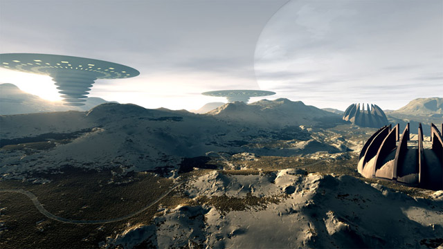
That's in fact the beauty of the technique - an incredibly simple code that produces interesting images. It's perfect for small size demos, that's why it has been used so much (think in Hymalaya/TBC or Ixaleno/rgba - the image below this text, which is created from a 4 kilobytes executable). In fact you can code a basic prototype in few minutes (Ixaleno was pretty much done in one day, coded from scratch during 2007 Christmas; then of course I had to spend some extra days tunning the colors etc, but that's another story. The purpose of this article is not to generate interesting terrains or landscapes (see articles like the one on advanced value noise), but how to render those with the simple raymarching algorithm.
The concept
The basic idea is to have a height function y = f(x,z) that defines for each 2d point in the plane (x,z) the height of the terain at that point.
f(x,z) = 2
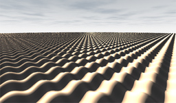
f(x,z) = sin(x)�sin(z)
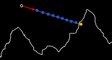
Once you have such a function f(x,z), the goal is to use a raytracing setup to render the image and do other effects as shadows or reflections. That means that for a given ray with some starting point in space (like the camera position) and a direction (like the view direction) we want to compute the intersection of the ray and the terrain f. The simplest approach is to slowly advance in the ray direction in small steps, and at each stepping point determine if we are above of below the terrain level. The image below shows the process. We start at some point in the ray close to the camera (the leftmost blue point in the image). We evaluate the terrain function f at the current x and z coordinates to get the altitude of the terrain h:h = f(x,z). Now we compare the altitude of the blue sampling point y with h, and we realize that y > h, or in other words, that the blue point is above the mountains. So, we step to the next blue point in the ray, and we repeat the process. At some point, perhapse, one of the sampling point will fall below the terrain, like the yellow point in the image. When that happens, y < h, and we know our ray crossed the terrain surface. We can just stop here and mark the current yellow point as the intersection point (even if we know it's slightly further than the real intersection point), or perhaps take the last blue point as interesection point (slightly closer than the real intersection) or the average of the last blue and yellow points.
bool castRay( const vec3 & ro, const vec3 & rd, float & resT )
{
const float dt = 0.01f;
const float mint = 0.001f;
const float maxt = 10.0f;
for( float t = mint; t < maxt; t += dt )
{
const vec3 p = ro + rd*t;
if( p.y < f( p.x, p.z ) )
{
resT = t - 0.5f*dt;
return true;
}
}
return false;
}
As you can see the code is terribly simple. There are many optimizations and improvements possible of course. For example, the accuracy of the intersection can be done more accurately by doing a linear approximation of the terrain altitudes between the blue and yellow points and compute the analytical intersection between the ray and the idealized terrain.
The other optimization is to note that as the marching moves the potential intersection point further and further (the bigger t becomes), the less important the error becomes, as geometric details get smaller in screen space as they get further from the camera. In fact, details decay inverse-linearly with the distance, so we can make our error or accuracy dt linear to the distance. This saves lot of rendering time and gives more uniform artifactas than the naive approach. This trick is described in several places, for example in the "Texturing And Modeling - A Procedural Approach" book.
bool castRay( const vec3 & ro, const vec3 & rd, float & resT )
{
const float dt = 0.01f;
const float mint = 0.001f;
const float maxt = 10.0f;
float lh = 0.0f;
float ly = 0.0f;
for( float t = mint; t < maxt; t += dt )
{
const vec3 p = ro + rd*t;
const float h = f( p.xz );
if( p.y < h )
{
// interpolate the intersection distance
resT = t - dt + dt*(lh-ly)/(p.y-ly-h+lh);
return true;
}
lh = h;
ly = p.y;
}
return false;
}
Variation of the basic code to suport linear interpolation of the terrain
bool castRay( const vec3 & ro, const vec3 & rd, float & resT )
{
float dt = 0.01f;
const float mint = 0.001f;
const float maxt = 10.0f;
float lh = 0.0f;
float ly = 0.0f;
for( float t = mint; t < maxt; t += dt )
{
const vec3 p = ro + rd*t;
const float h = f( p.xz );
if( p.y < h )
{
// interpolate the intersection distance
resT = t - dt + dt*(lh-ly)/(p.y-ly-h+lh);
return true;
}
// allow the error to be proportinal to the distance
dt = 0.01f*t;
lh = h;
ly = p.y;
}
return false;
}
Variation of the basic code to suport linear interpolation of the terrain and adaptive error
So the complete algorithm to build an image is simple. For every pixel of the screen construct a ray that starts at the camera position that passes through the pixel location as if the screen was right in front of the viewer, and cast the ray. Once the intersection point is found, the color of the terrain must be gathered, the shaded, and a color must be returned. That's what the terrainColor() functions must do. If there is no intersection with the terrain, then the right color must be computed for the sky. So, the main code looks like this:
void renderImage( vec3 *image )
{
for( int j=0; j < yres; j++ )
for( int i=0; i < xres; i++ )
{
Ray ray = generateRayForPixel( i, j );
float t;
if( castRay( ray.origin, ray.direction, t ) )
{
image[xres*j+i] = terrainColor( ray, t );
}
else
{
image[xres*j+i] = skyColor();
}
}
}
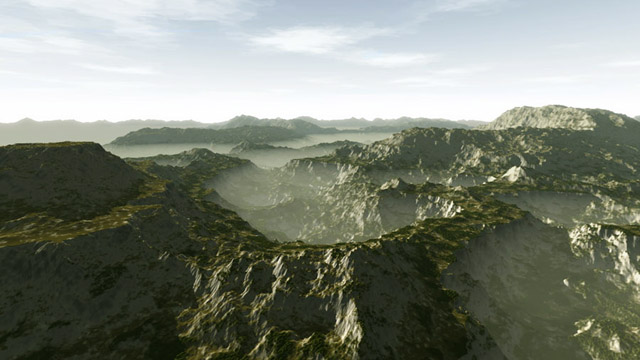
An image rendered with the algorithm in the left. Click to enlarge
Usually terrainColor() will need to compute first the intersection point p, then compute the normal to the surface n, do some lighting/shading s based on that normal (even cast some shadow ray by using the castRay() function for doing some shadows), decide the color of the terrain surface m at the intersection point, combine the shading information with it, and probably do some fog calculations. Something like this:
vec3 terrainColor( const Ray & ray, float t )
{
const vec3 p = ray.origin + ray.direction * t;
const vec3 n = getNormal( p );
const vec3 s = getShading( p, n );
const vec3 m = getMaterial( p, n );
return applyFog( m * s, t );
}
The normal can be computed as usual with the central differences method:
vec3 getNormal( const vec3 & p )
{
return normalize( vec3( f(p.x-eps,p.z) - f(p.x+eps,p.z),
2.0f*eps,
f(p.x,p.z-eps) - f(p.x,p.z+eps) ) );
}
The getShading() function will probably need to compute some diffuse lighting from a powerfull yellowish directional light that simulates the sun, and a dimmer bluish area light simulating the sky dome (some sort of ambient occlusion). Doing shadows in a terrain is interesting since many optimizations can be done. One such trick is to compute soft shadows for free by computing how depth the shadow ray went into the terrain. By smoothstep()-ing this amount one can control the penumbra of the mountains.
To get the material of the surface, usually the altitude and slope of the mountains and the point p is taken into account. For example, at high altitudes you can return a white color and at low altitudes some brown or grayish. The transition can be controled again with some smoothstep() functions. Just remember to randomize (with perlin noise) all the parameters so the transitions are not constant and so it all looks more natural. It's a good idea to take the slope of the terrain into account also, since snow and grass usually only stay on flat surfaces. So, if the normal is very horizontal (ie, n.y is small) it's a good idea to blend with some grey or brown color, to remove snow or grass. That makes the textures naturally fit the terrain, and the image gets richer.
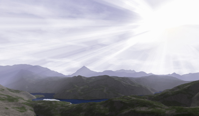
And old image, made in 2002. Click to enlarge

And old image, made in 2002. Click to enlarge