


Intro
Computing axis aligned bounding boxes (AABBs) of different geometrical primitives is useful for collision detection and for rendering algorithms. In particular, disks are a common primitive used for splatting and global illumination lighting algorithms, for representing distant geometry and for point cloud rendering. So, being able to compute the tightest possible axis aligned bounding box of an arbitrarily oriented disk is pretty important, especially if it can be done quickly and analytically without having to loop over the perimeter of the disk. Fortunately, such a close form expression exists.
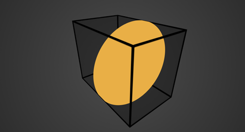
Mathematically perfect (tightest) axis aligned bounding box of a disk
Maths
Luckily for us computing the bounding box of an arbitrarily oriented ellipse in 3D space can be done exactly if the ellipse is defined by its center, radius and two orthonormal tangent axes. The derivation is easy, you can find it in this other article that I wrote some time ago, the result been:

where u and v are the axes of the ellipse.
The only problem is that disks are usually defined by a single orientation vector (or normal) rather than two (different sized) axes. One way to work around this is to stick with our disk normal and then compute two orthonormal vectors to it by cross-producting the normal with some non-parallel vector. However, while this works well, it seems like a waste of compute and it's mathematically inelegant (and therefore unsatisfactory), for it seems it shouldn't be necessary to use arbitrary vectors to perform a pretty deterministic computation.
My solution in order to do so was first noting that crossing the normal vector with either of the canonical i, j or k axes produces a different pair of axes and a different mathematical expression, but the three of them should land on the same numerical bounding box result, for the disk is unique. This means that actually developing the three computations into the three different expressions and combining them together into a single one should still be a valid solution, but should remove all the asymmetries in the terms you get otherwise by choosing only one of the three axis.
So, let's see. For a given disk orientation or normal n = (x, y, z), constructing the basis vectors u and v crossing n with the three canonical axes (1,0,0), (0,1,0) and (0,0,1) produces the following:
ui = (1,0,0) × (x,y,z) vi = ui × (x,y,z)
uj = (0,1,0) × (x,y,z) vj = uj × (x,y,z)
uk = (0,0,1) × (x,y,z) vk = uk × (x,y,z)
which, taking into account that |n| = 1, would result in the following u and v axis vectors:
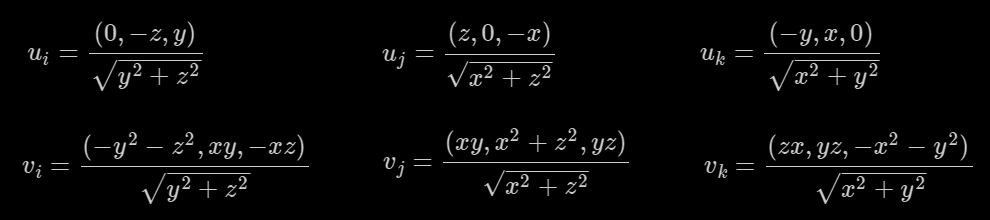
In order to get the bounding box extents, we'd have to choose one of these solutions for i, j or k and square and add the three x, y and z components of u and v, before doing the last square root. Since we decided we'd instead use the three of them and add them together, let's do so. What we get before square rooting and averaging down (dividing by 3) is:

which after much mathematical manipulation searching for symmetry in the terms, and after fair amount of cancellations and simplifications, I arrived to some pretty decently coordinate-independent solution for the x coordinate, which Cleve Ard simplified even further:
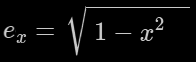
The y and z components of the bounding box extent can be obtained similarly. Then the three components can be expressed as a single vector calculation, assuming that vectors get multiplied and squared component-wise (not dotted or crossed):
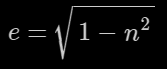
Which is indeed a particular case of the formula for the ellipse that we started with for the case in which |u| = |v| = 1. Hence, the final bounding box for our disk or radius r, centered at position c and oriented to face the direction n, is

Code
The code is a direct implementation of the formula above, and exploits the component-wise multiplication of vectors. The only note here is that if you want to be smart you can encode a disk described by a position, a normal and a radius in 6 floats instead of 7, since you can encode the radius of the disk in the length of the normal. However, for clarity the code below assumes the straightforward 7 floats description of a disk:
struct bound3
{
vec3 mMin;
vec3 mMax;
};
// bounding box for a disk defined by cen(ter), nor(mal), rad(ius)
bound3 DiskAABB( in vec3 cen, in vec3 nor, float rad )
{
vec3 e = rad*sqrt( 1.0 - nor*nor );
return bound3( cen-e, cen+e );
}
This realtime visual shows the bounding box computed by the code above: https://www.shadertoy.com/view/ll3Xzf
Beyond disks
A nice side effect of this efficient and exact bounding box computation for disks is that we can apply it to the computation of arbitrarily oriented cylinders and cones as well, by noting that the bounding box of such a shapes is the bounding box of the bounding boxes of their caps.
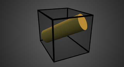
Mathematically perfect (tightest) axis aligned bounding box of a cylinder
Since the maths are basically the same, I'll simply drop the code for the cylinder:
// bounding box for a cylinder defined by points pa and pb, and a radius ra
bound3 CylinderAABB( in vec3 pa, in vec3 pb, in float ra )
{
vec3 a = pb - pa;
vec3 e = ra*sqrt( 1.0 - a*a/dot(a,a) );
return bound3( min( pa - e, pb - e ),
max( pa + e, pb + e ) );
}
and for the cone:
// bounding box for a cone defined by points pa and pb, and radii ra and rb
bound3 ConeAABB( in vec3 pa, in vec3 pb, in float ra, in float rb )
{
vec3 a = pb - pa;
vec3 e = sqrt( 1.0 - a*a/dot(a,a) );
return bound3( min( pa - e*ra, pb - e*rb ),
max( pa + e*ra, pb + e*rb ) );
}
You can find the realtime version with this code above in action here: https://www.shadertoy.com/view/ll3Xzf and https://www.shadertoy.com/view/WdjSRK