


Intro
This is one of the very first things I coded in OpenGL when I started learning in 2002. In fact, this effect, or trick, or technique is one of the examples of the OpenGL manual, so I didn't invent anything, just follow the explanation and code it. Cellular patterns, or more exactly, Voronoi diagrams, appear in computer graphics and robotics often. Given a set of features (points, lines, circles, objects, whatever), such a diagram represents the distance to the closest feature for a given distance metric (for example, the regular euclidean distance). When representing the distances with colors one gets the usual cellular textures, very usefull as primitive for procedural texture generation (for rocks, tiles, trees, skin, etc etc). This article is not about how to nicely create this patterns or how to use them in procedural texture generation, but on how to render simple Voronoi diagrams using OpenGL in realtime as described in the OpenGL manual, and as I tested it in 2002.
The images on the right are the result of runing the OpenGL experiment. You can download it here. The first image is the direct visualization of the results of the algorithm. The second one shows a variation where the color of each cell is taken based on a bitmap. The third one shows the cell id as a color, and the last one is a version where the distance metric has been changed. They all run in realtime of course, they could even run fullspeed in software rendering mode, it's a very cheap technique. In fact it runs in linear time, instead of the other O(n⋅log(n)) versions. The problem is it's sampled and not analytical, neither it is perfect. But well, for democoders that might not be a problem.
The idea is very imaginative but simple, I think I read about it in the OpenGL Red Book: use the zbuffer of the graphics card to track the closest distance from any pixel to any of the features. Each feature expands a distance field around it. The shape of the field depends on the metric used of course. If one uses the regular euclidean distance, the distance decreases equally in all directions in concentric circles. If you visualize the distance to a point with such a metric, you get a circular gradient, or if displayed as a heighfield, a cone with it's apex at the location of the point. As you add more points to the plane, each of them expands it's own distance field (the circular gradient/cone). The Voronoi diagram must compute, for each pixel, the minimun of all these gradients/cones. And we can do that with the zbuffer, since the zbuffer is designed exactly for that, to track the minimun of the distances to geometry. So, what we have to do is to render one cone for each feature point with the zbuffer enabled. Et voila, we have our diagram. If we asign constant color to the cones we will have a something like the third image shown in this article. If we want to see the real Voronoi diagram we have to render the apex of the cone in black (since the distance there is zero) and full white in the base of the cone. The cone needs to have a 45 degree angle of course, so distances in 2d map to linear distances in the z axis too (where the zbuffer does it's job). Well, the complete description of the algorithm is in the OpenGL manual as said, I'm not goint to duplicate it. So, Image 1 is computed with the direct implementation of the algorithm. In Image 3, each cone has a constant unique color, so you can see the individual cells very easily. The black lines are created as a postprocess effect. Image 2 is a combination of the two previous methods. Each cone has a constant color taken from sampling a bitmap at the feature location, and it has a little color modulation based on the first technique. Image 4 is what you get when you don't use a cone for rendering the distance field, but a pyramid: features expand rectangular fields.
The code goes like this:
void renderCellularEffect( float time )
{
// set 2d mode
glMatrixMode( GL_PROJECTION );
glLoadIdentity();
glMatrixMode( GL_MODELVIEW );
glLoadIdentity();
// clear the buffers
glClear( GL_COLOR_BUFFER_BIT|GL_DEPTH_BUFFER_BIT );
glEnable( GL_DEPTH_TEST );
// render the cells
const int numCells = 100;
int sem = 134;
for( j=0; j < numCells; j++ )
{
// move the cell on the screen
float x = cosf( sfrand(&sem)*3.14f + sfrand(&sem)*time );
float y = cosf( sfrand(&sem)*3.14f + sfrand(&sem)*time );
// render cone (can be optimized of course)
glBegin( GL_TRIANGLE_FAN );
glColor4f( 0.0f, 0.0f, 0.0f, 1.0f );
glVertex3f( x, y, 1.0f );
glColor4f( 1.0f, 1.0f, 1.0f, 1.0f );
for( i=0; i < 48; i++ )
{
const float an = (6.28318f/47.0f)*(float)i;
glVertex3f( x+cosf(an), y+sinf(an), -1.0f );
}
glEnd();
}
}
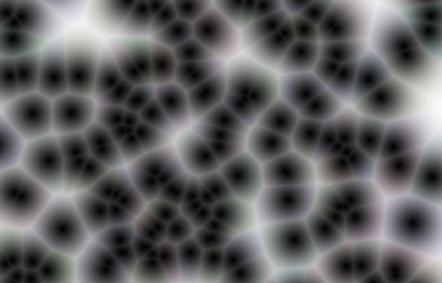
Image 1. The classical cellular texture
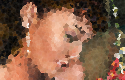
Image 2. A modified version using a bitmap as cell color

Image 3. A modified version, using the cell id as color

Image 4. A modified version, using a different distance metric